

ACCESS FOR LIFE
Access this course forever. Watch the videos and review the lessons anytime, at your own pace

CERTIFICATE
After finishing the course you will get your certificate of completion

RESOURCES
You will get all the scripts, programs, examples and quizzes of the course

QUESTIONS
I will solve all your questions throughout the course
- 1.1 – 🎬 Introduction to composite materials
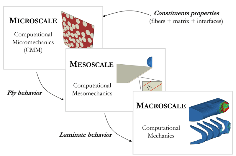
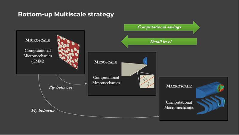
- 2.1 – 🎬 The Bottom-up Multiscale strategy
- 2.2 – Structure of the course
- 1.1 – Introduction to composite materials
- 1.1.1 – 🎬 Introduction to CMM
- 1.2 – Numerical strategies for CMM
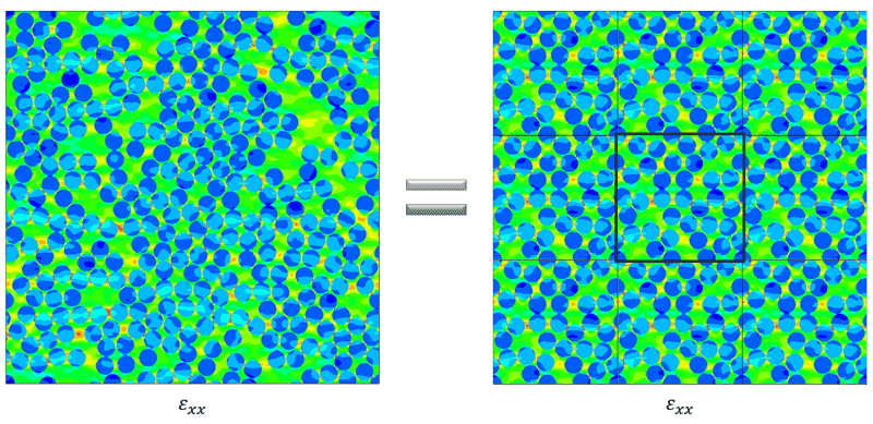
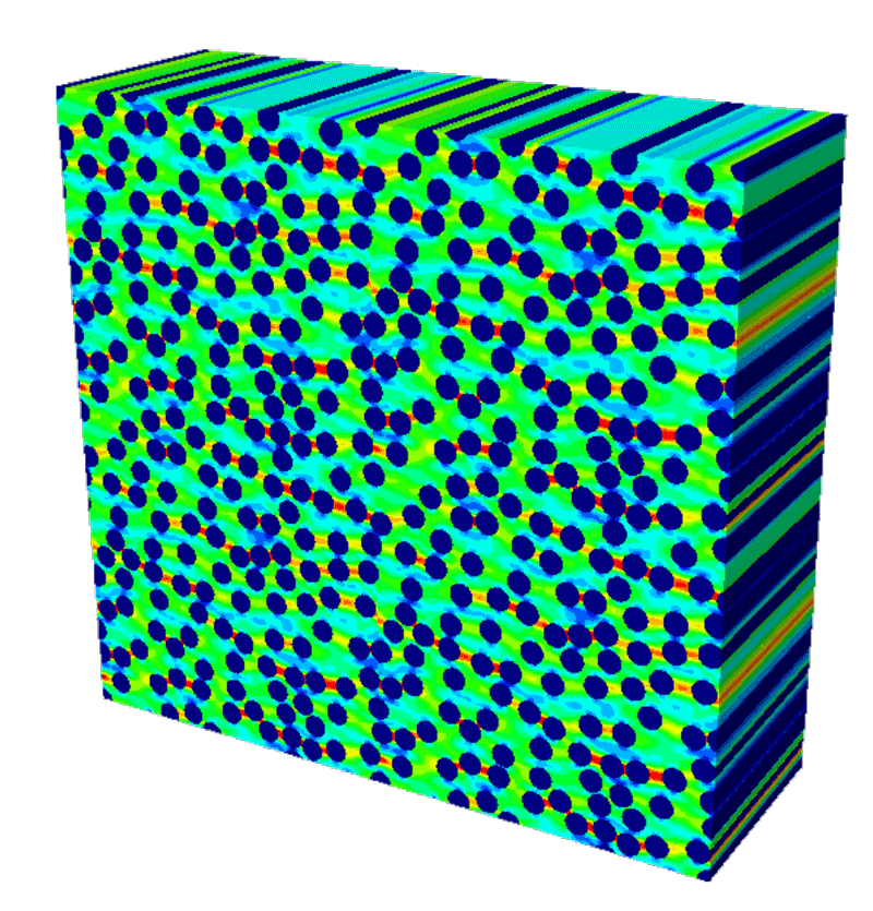
- 1.2.1 – 🎬 CMM: Periodic RVEs
- 1.3 – Structure of the chapter
- 2.1 – Development of a unit cell model
- 2.1.1 – 🎬 Presentation of the model
- 2.1.2 – 🎬 Creation of the part
- 2.1.3 – 🎬 Meshing the part
- 2.1.4 – 🎬 Assembly and boundary conditions
- 2.1.5 – 🎬 Job and first results
- 2.2 – Periodic boundary conditions (PBC)
- 2.2.1 – 🎬 Introduction to PBC
- 2.2.2 – 🎬 Creation of a 2D unit cell
- 2.2.3 – 🎬 Definition of equations in Abaqus
- 2.2.4 – 🎬 Script to generate PBC in 2D (1/2)
- 2.2.5 – 🎬 Script to generate PBC in 2D (2/2)
- 2.2.6 – 🎬 Including PBC in the model
- 2.2.7 – 🎬 Definition of PBC in 3D
- 2.2.8 – 🎬 Computing the Poisson ratios using master nodes
- 2.3 – Automatic generation of the FE model using a Python script
- 2.3.1 – 🎬 Script of the unit cell model (1/4)
- 2.3.2 – 🎬 Script of the unit cell model (2/4)
- 2.3.3 – 🎬 Script of the unit cell model (3/4)
- 2.3.4 – 🎬 Script of the unit cell model (4/4)
- 2.3.5 – 🎬 Script of the RVE model (1/3)
- 2.3.6 – 🎬 Script of the RVE model (2/3)
- 2.3.7 – 🎬 Script of the RVE model (3/3)
- 2.4 – Algorithm to generate random microstructures
- 2.4.1 – 🎬 Theory: Random Sequential Absorption algorithm
- 2.4.2 – 🎬 Implementation in a script (1/2)
- 2.4.3 – 🎬 Implementation in a script (2/2)
- 2.4.4 – 🎬 Visualization of the microstructures
- 2.4.5 – 🎬 Jamming limit and tolerance distance
- 2.4.6 – 🎬 Some visualization tips
- 2.4.7 – 🎬 Transformation of the RSA algorithm into a function
- 2.4.8 – 🎬 Integration of RSA in the FEA worflow
- 2.4.9 – 🎬 Advanced scripting: Exceptions
- 2.5 – Computing the elastic properties of the UD ply
- 2.5.1 – 🎬 How to compute the elastic properties
- 2.5.2 – 🎬 Computing the elastic properties in Abaqus
- 2.5.3 – 🎬 Definition of the normal loading cases
- 2.5.4 – 🎬 Definition of the shear loading cases
- 2.5.5 – 🎬 Automating the postprocess (1/2)
- 2.5.6 – 🎬 Automating the postprocess (2/2)
- 2.5.7 – 🎬 Analysis of the results: Elastic properties
- 2.5.8 – 🎬 Simulation of thermal expansion
- 3.1 – Limitations of the periodic RVE models
- 3.1.1 – 🎬 Periodic RVEs have limits
- 3.2 – Inelastic deformation of the constituents
- 3.2.1 – 🎬 Micromechanical inelastic deformation mechanisms
- 3.2.2 – 🎬 Matrix: Plastic deformation
- 3.2.3 – 🎬 Interface: Cohesive Zone Model
- 3.3 – Modifications in the RVE model
- 3.3.1 – 🎬 Preparation of a script to generate the new model
- 3.3.2 – 🎬 Insertion of cohesive elements along the interfaces (1/3)
- 3.3.3 – 🎬 Insertion of cohesive elements along the interfaces (2/3)
- 3.3.4 – 🎬 Insertion of cohesive elements along the interfaces (3/3)
- 3.3.5 – 🎬 Convergence issues and final touches
- 3.4 – Loading cases
- 3.4.1 – 🎬 Transverse tension
- 3.4.2 – 🎬 Review of transverse tension case
- 3.4.3 – 🎬 Transverse compression
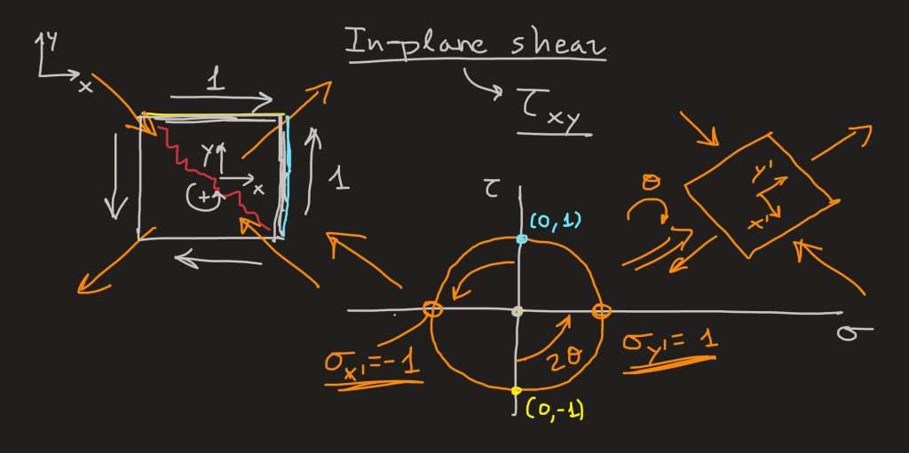
- 3.4.4 – 🎬 Longitudinal shear
- 3.4.5 – 🎬 Transverse shear
- 3.4.6 – 🎬 Residual thermal stresses
- 3.5 – Solving common problems
- 3.5.1 – 🎬 Issue #1: PBC not working
- 3.5.2 – 🎬 Issue #2: Instance not meshed
- 3.5.3 – 🎬 Issue #3: Invalid mesh
- 4.1 – Computational Micromechanics is more than RVEs
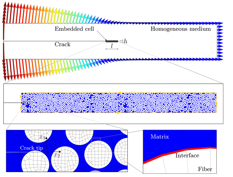
- 4.1.1 – 🎬 Alternatives to periodic RVEs
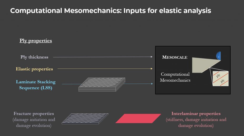
- 1.1 – 🎬 Introduction to Computational Mesomechanics
- 1.2 – 🎬 Naming convention of laminate stacking sequences (LSS)
- 1.3 – Structure of this chapter
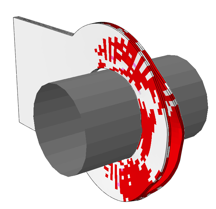
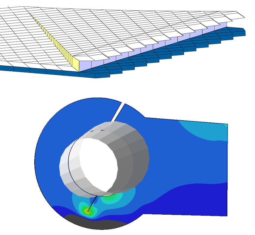
- 2.1 – Development of the elastic FE model of the pinned joint
- 2.1.1 – 🎬 Presentation of the model
- 2.1.2 – 🎬 Pinned joint: Part
- 2.1.3 – 🎬 Pinned joint: Mesh
- 2.1.4 – 🎬 Pinned joint: Material
- 2.1.5 – 🎬 Pinned joint: Assembly
- 2.1.6 – 🎬 Pinned joint: Contact
- 2.1.7 – 🎬 Pinned joint: Rigid pin
- 2.1.8 – 🎬 Pinned joint: Boundary conditions
- 2.1.9 – 🎬 Pinned joint: Results
- 2.2 – Automating the generation of the FE model using Python script
- 2.2.1 – 🎬 Python script of the pinned joint: Sketch and part
- 2.2.2 – 🎬 Python script of the pinned joint: Sets and partitions of the plies
- 2.2.3 – 🎬 Python script of the pinned joint: More partitions
- 2.2.4 – 🎬 Python script of the pinned joint: Mesh, material and sections
- 2.2.5 – 🎬 Python script of the pinned joint: From assembly to job
- 2.2.6 – 🎬 Python script of the pinned joint: Final
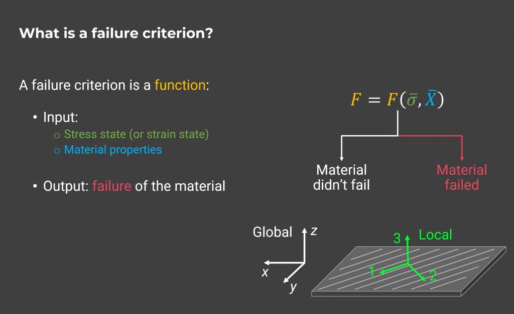
- 3.1 – Introduction to failure criteria of materials
- 3.1.1 – 🎬 Fundamentals of failure criteria of materials
- 3.1.2 – 🎬 Failure criteria of composite materials
- 3.2 – Failure criteria of composites in Abaqus
- 3.2.1 – 🎬 Modification of the model: Hashin material properties
- 3.2.2 – 🎬 Modification of the model: Mesh, section and output
- 3.2.3 – 🎬 Including the Hashin criterion in the script
- 4.1 – Introduction to damage of composite materials at the mesoscale
- 4.1.1 – 🎬 Modeling damage in mesomechanical models
- 4.2 – Modeling intralaminar damage
- 4.2.1 – 🎬 Damage evolution parameters in Abaqus
- 4.2.2 – 🎬 Damage and loss of convergence
- 4.2.3 – 🎬 Stabilizing the model through viscous dissipation
- 4.2.4 – 🎬 Hashin damage variables
- 4.2.5 – 🎬 Hashin damage: Python script
- 4.2.6 – 🎬 Understanding damage evolution in CDM
- 4.2.7 – 🎬 Element size dependence in CDM
- 4.3 – Modeling interlaminar damage I (cohesive elements)
- 4.3.1 – 🎬 Introduction to interlaminar damage
- 4.3.2 – 🎬 Interlaminar properties
- 4.3.3 – 🎬 Making the partitions for the cohesive elements
- 4.3.4 – 🎬 Finishing the model with cohesive elements
- 4.3.5 – 🎬 Results and damage initiation criterion
- 4.4 – Convergence, solvers and steps
- 4.4.1 – 🎬 Implicit dynamic step
- 4.4.2 – 🎬 Implicit vs. Explicit
- 4.4.3 – 🎬 Explicit step: Abaqus/CAE
- 4.4.4 – 🎬 Explicit step: Script
- 4.4.5 – 🎬 Stable time increment
- 4.5 – Fracture Process Zone (FPZ)
- 4.5.1 – 🎬 Definition of fracture process zone
- 4.5.2 – 🎬 How to use a coarse mesh along the FPZ
- 4.5.3 – 🎬 Implications and limitations tuning the FPZ
- 4.5.4 – 🎬 Results: delamination
- 4.6 – Modeling interlaminar damage II (cohesive surfaces)
- 4.6.1 – 🎬 Introduction to cohesive surfaces modeling
- 4.6.2 – 🎬 Definition of cohesive contact in Abaqus/Explicit
- 4.6.3 – 🎬 Scripting the cohesive contacts
- 4.6.4 – 🎬 Cohesive elements vs. Cohesive surfaces
- 5.1 – 🎬 Summary
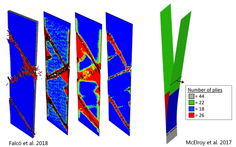
- 5.2 – 🎬 State of the art: Techniques and theories
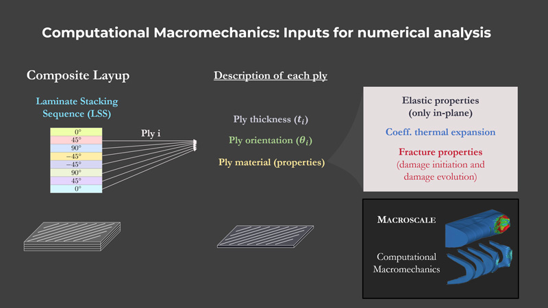
- 1.1 – 🎬 Introduction to Computational Macromechanics
- 1.2 – Structure of this chapter
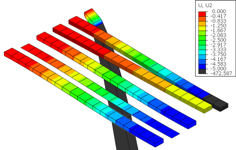
- 2.1 – Development and analysis of equivalent models with different element types
- 2.1.1 – 🎬 Presentation of the model
- 2.1.2 – 🎬 Case 1: C3D8R x 1 (preprocess)
- 2.1.3 – 🎬 Case 1: C3D8R x 1 (results)
- 2.1.4 – 🎬 Case 2: C3D8R x 5
- 2.1.5 – 🎬 Case 2: C3D8R x 5 (verification)
- 2.1.6 – 🎬 Case 3: C3D8 x 5
- 2.1.7 – 🎬 Case 4: SC8R
- 2.1.8 – 🎬 Case 5: S4R
- 2.1.9 – 🎬 Visualization of results in shell elements
- 2.1.10 – 🎬 Summary and one more case
- 2.2 – Analytical solution of the doubly-clamped beam
- 2.2.1 – Solving the problem
- 3.1 – Definition of Composite Layups in Abaqus
- 3.1.1 – 🎬 Introduction to Composite Layups in Abaqus
- 3.1.2 – 🎬 Example 1: Unidirectional laminate (preprocess)
- 3.1.3 – 🎬 Example 1: Unidirectional laminates (analysis)
- 3.1.4 – 🎬 Example 2: Cross-ply laminate
- 3.1.5 – 🎬 Example 3: Cross-ply hybrid laminate
- 3.1.6 – 🎬 Example 4: Non-symmetric cross-ply
- 3.1.7 – 🎬 Example 5: Anti-symmetric balanced laminate
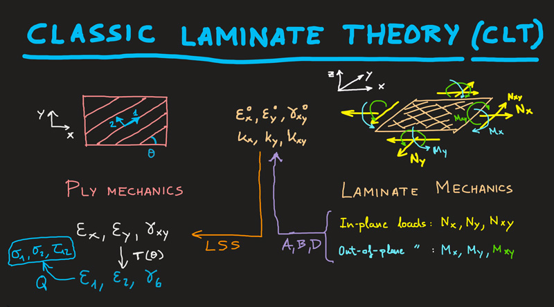
- 3.2 – Classic Laminate Theory (CLT)
- 3.2.1 – 🎬 Introduction to CLT
- 3.2.2 – 🎬 Ply Mechanics
- 3.2.3 – 🎬 Laminate Mechanics
- 3.2.4 – 🎬 Laminate matrices under in-plane loading
- 3.2.5 – 🎬 Laminate matrices under out-of-plane loading
- 3.2.6 – 🎬 Symmetric laminates and some remarks
- 3.3 – Verification of numerical models
- 3.3.1 – 🎬 Putting CLT into practice
- 3.3.2 – 🎬 Analyses of symmetric laminates (ex. 1, 2 & 3)
- 3.3.3 – 🎬 Analysis of non-symmetric cross-ply (ex 4)
- 3.3.4 – 🎬 Analysis of anti-symmetric balanced laminate (ex 5)
- 3.3.5 – 🎬 How to get the A, B, D matrices in Abaqus
- 3.4 – Effective laminate moduli
- 3.4.1 – 🎬 In-plane laminate moduli
- 3.4.2 – 🎬 Out-of-plane laminate moduli
- 4.1 – Introduction and analysis of the initial design
- 4.1.1 – 🎬 Pressurized vessel: Introduction
- 4.1.2 – 🎬 Pressurized vessel: Part and mesh
- 4.1.3 – 🎬 Pressurized vessel: Material and section
- 4.1.4 – 🎬 Pressurized vessel: BCs and job
- 4.1.5 – 🎬 Pressurized vessel: Preliminary analysis
- 4.1.6 – 🎬 Pressurized vessel: Cross-ply laminate
- 4.1.7 – 🎬 Custom field output
- 4.2 – Optimization of the laminate
- 4.2.1 – 🎬 Optimality vs. Versatility
- 4.2.2 – 🎬 Design of a balanced laminate
- 4.2.3 – 🎬 Modification of the original laminate
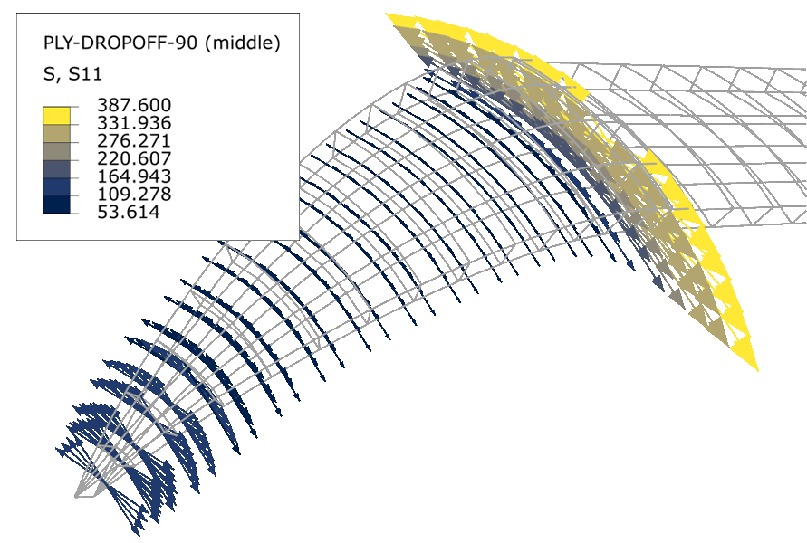
- 4.2.4 – 🎬 Further optimization: Ply drop-off
- 4.3 – New ply failure criteria: LaRC05
- 4.3.1 – 🎬 How are jobs run by Abaqus?
- 4.3.2 – 🎬 LaRC05: Introduction
- 4.3.3 – 🎬 LaRC05: Parameters
- 4.3.4 – 🎬 Including the LaRC05 criterion in the input file
- 4.3.5 – 🎬 How to run a model from the input file: 2 methods
- 4.4 – Thermal residual stresses
- 4.4.1 – 🎬 Introduction to thermal stress
- 4.4.2 – 🎬 Thermal residual stresses in composite laminates
- 4.4.3 – 🎬 Thermal stresses in Abaqus
- 4.5 – Sandwich laminate for cryogenic applications I
- 4.5.1 – 🎬 Design proposal
- 4.5.2 – 🎬 Sandwich laminate: Part
- 4.5.3 – 🎬 Sandwich laminate: Mesh
- 4.5.4 – 🎬 Sandwich laminate: Materials and sections
- 4.5.5 – 🎬 Sandwich laminate: Full model
- 4.5.6 – 🎬 Sandwich laminate: Results (only pressure)
- 4.6 – Sandwich laminate for cryogenic applications II
- 4.6.1 – 🎬 Modeling the cooling down to cryogenic conditions
- 4.6.2 – 🎬 Analysis of the final results
- 4.6.3 – 🎬 Final comments
- 5.1 – 🎬 Conclusions
- 5.2 – 🎬 Macromechanics or Mesomechanics
- 1.1 – 🎬 State of the art across the scales
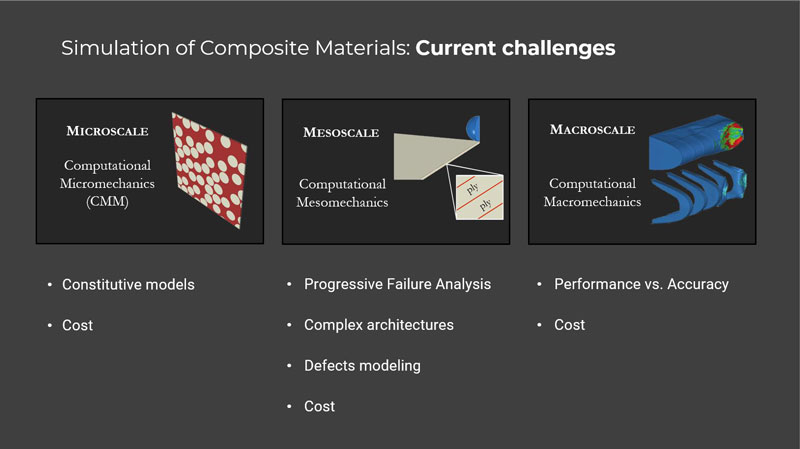
- 2.1 – 🎬 Current challenges and opportunities
“Thank you, Miguel! It was very detailed and useful, and I found all the answers to all my questions. I had a gap in fracture mechanics, but now I have a wide knowledge that allows me to effectively model the behavior of a composite structure. Thank you very much for your efforts and very good presentation. Looking forward to the next one!”

Let me first congratulate with you for the AWESOME content you are putting together: I can say that there’s nothing up to this level to date, so please keep going! As a young CAE simulation engineer, I have always had to find the way by myself to shed more light on topics not covered while at Uni or to get a reasonably correct answer to some of the many questions I’ve been posing myself during the past years on various problems regarding materials modelling, failure theories applicability, fatigue and contact mechanics. I really want to thank you for the massive effort you underwent to provide me and other people with such valuable knowledge

“I have learned a lot from your composite modelling course. My knowledge on FEA has increased a lot after taking your course. Will there be a course on writing subroutines like UMATs?”

“I have just completed the Simulation of Composite Materials with Abaqus course. I have to say this has been such a great course from the very beginning till the end. Very well presented, explained and structured, combining theory, references, methodology, and practical case studies, with the thinking process capturing the essence of the topic. This course and the knowledge you share makes me want to know even more and dive deeper. I have really enjoyed this course and I am hoping to see more content and courses on composites. I would highly recommend this course. The value and content that is presented in the course saves countless hours of research and struggle"

“I started your course on composites. You saved my life. I can now speed up a lot of my research. It was the best day of my PhD until now. Thanks a lot!”

“It’s good to start discovering the ability to automate any sort of operations in Abaqus by means of Python scripting. Thank you Miguel Herraez Matesanz for this wonderful course”